Vector data cubes in Xarray

Software Engineer
This is a blog version of a webinar that took place on August 27, 2024. Here’s a video of that webinar:
Geospatial datasets representing information about real-world features such as points, lines, and polygons are increasingly large, complex, and multidimensional. They are naturally represented as vector data cubes: n-dimensional arrays where at least one dimension is a set of vector geometries. The Xarray ecosystem now supports vector data cubes thanks to Xvec, a package designed for working with vector geometries within the Xarray data model 🎉. For those familiar with GeoPandas, Xvec is to Xarray as GeoPandas is to Pandas.
This blog post is geared toward analysts working with geospatial datasets. We introduce vector data cubes, discuss how they differ from raster data cubes, and describe the analytical opportunities they enable. We demonstrate these ideas by constructing a vector data cube from ERA5 reanalysis data sampled at a set of geometries representing points of interest.
Background
Raster data cubes and vector dataframes
The Python ecosystem has robust tools built to work with both raster and vector data. Geospatial raster data are typically stored as multi-dimensional arrays, with dimensions such as [x, y] or [longitude, latitude] representing the spatial domain of the dataset. For example, a satellite image usually covers a swath of area of the Earth’s surface with either latitude,longitude, or x,y dimensions. Raster data cubes can have additional dimensions such as time and a vertical dimension such as height or level. These data are typically stored on disk in array-based formats such as NetCDF, Zarr, or GeoTIFF, and analyzed with powerful tools like Xarray and Numpy. In contrast, geospatial vector data, which model real-world features like rivers, counties, and buildings as geometry objects, are typically stored as tables and formatted on disk in vector-specific containers like GeoJSON, Shapefile, or GeoParquet. In memory, geometries are commonly represented as Shapely geometries, and vector dataframes are analyzed using the GeoPandas library.
The key difference: raster data is viewed as a cube, while vector data is (mostly) viewed as a dataframe. Both of these are powerful and functional formats, but they are optimized for different types of operations. Thus, framing raster data as cubes and vector data as tables can influence how we, as analysts, both think about our data, and the analytical questions we ask with it. Further, analysts commonly want to merge the raster and vector data worlds; for instance, sampling a raster data cube at a set of points described by a vector dataframe.
The drawbacks of dataframes
Some data is more naturally represented as a multi-dimensional cube. Consider a collection of weather stations that record temperature and windspeed. These measurements are stored in the columns of a geopandas.GeoDataFrame, while the coordinates of each weather station are stored as Shapely Point geometries in a geometry column. We can quickly access a lot of information and ask questions such as “how do temperatures vary across the elevation range covered by the weather stations”, and “where are windspeeds highest?” But, each time the weather station records a measurement, we get a new set of data for each variable. How should that new data be incorporated into the GeoDataFrame? While there are ways of representing such multi-dimensional data in tabular form (see Pebesma, 2022), the column structure is still fundamentally one-dimensional, and these strategies all involve duplicating data along either the row or column dimension.
In the weather station example, the data are fundamentally two-dimensional ([location, time]) and must be flattened to fit into a dataframe. Contrast this to raster data cubes, where data is explicitly represented as multi-dimensional. In this data model, adding new dimensions is easy, and popular tools reflect this fundamental concept. What would it look like, and how would our workflows change, if vector data were also represented as a cube?
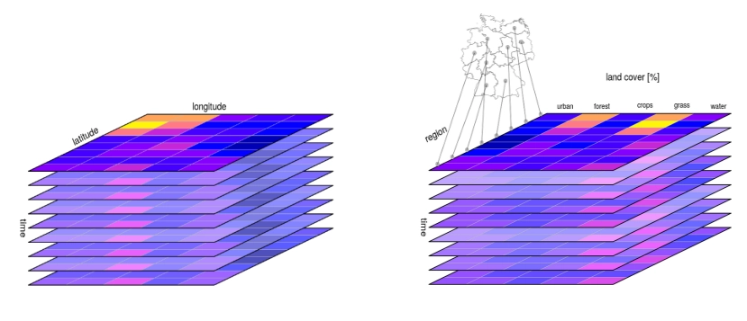
Example of a raster data cube (left) and vector data cube (right). The raster data cube has a gridded structure with latitude, longitude and time dimensions. The vector data cube has a dimension of geometries, a dimension of data variables and a time dimension. Source: R-Spatial: Data Cubes
What are vector data cubes?
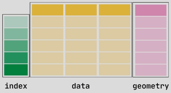
The defining characteristic of a vector dataframes is that the data are contained in a set of 1-D columns, and one or more columns contain vector geometries. Generalizing this structure leads us to vector data cubes. Vector data cubes are n-dimensional arrays with at least one dimension that is an array of geometries (Pebesma, 2022). Where the spatial domain of a raster object is a gridded extent (eg. rdc = {'x': [0,1,2,3,4,5,6,7,8,9], 'y':[0,1,2,3,4,5,6,7,8,9]}), the spatial domain of a vector data cube is an array of points, lines or polygons representing real-world features:
What can we do with vector data cubes?
Vector data cubes allow users to observe how geospatial features, or data associated with those features, change over time: for example, tracking areal extents such as forest boundaries and agricultural parcels, or data from non-stationary monitoring systems such as ocean data buoys. Important information about the sampling locations will be preserved as points or other geometries, making the result a vector data cube. A particularly exciting use case is sampling gridded raster data at a number of polygons of interest, going from a raster data cube covering a large spatial extent to a vector data cube containing only the spatial areas of interest, while preserving information about the spatial sampling. To illustrate, we will sample the ERA5 atmospheric reanalysis dataset at a number of point locations representing cities across Europe.
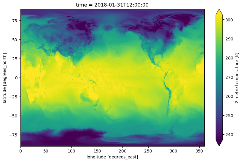
ERA5 is a dataset that provides estimates for 32 atmospheric variables for the entire globe for every 6-hour window from 1959 to 2022. We will use an ‘analysis-ready’ dataset, from WeatherBench2 which makes it possible to access ERA 5 data from Google Cloud Storage, letting us work with this dataset without downloading it to a local machine.
Assemble vector data cube
Below is a Jupyter notebook that demonstrates constructing a vector data cube by sampling a raster cube at a set of Point geometries.
Wrap up
Vector data cubes offer a natural way to manipulate and analyze n-dimensional data indexed along geometric dimensions, particularly with respect to spatial analytics. We look forward to seeing how the scientific community leverages vector data cubes to produce novel analytical workflows.
A few rough edges, such as plotting, remain around interoperability between Xarray vector data cubes and existing Xarray methods. Stay tuned for more updates to vector data cubes in Xarray, and check out the Xvec repository if you’re interested in getting involved.
Implementing vector data cubes is the result of hard work and development across the open-source community by a number of individuals and groups working on a range of packages. It’s exciting to see collaborative efforts in the open-source community that lead to significant breakthroughs and improvements to user experience.
Acknowledgments
- Many groups and individuals worked to make vector data cubes possible, the following individuals deserve special recognition for their efforts in coordinating and executing this project: Martin Fleischmann, Benoit Bovy, Mohammad Alasawedah.
- WeatherBench2 for analysis-ready ERA5 data
- HuggingFace datasets for global cities dataset
References
The R programming language also has strong support for vector data cubes, which inspired much of this work. For information about vector data cube software in R, check out the
starspackage, and for a very detailed background on vector data cubes, check out this post by Edzer Pebesma, astarsdeveloper.
Software Engineer