This is a blog version of a webinar that took place on April 16, 2024. Here’s a video of that webinar:

---

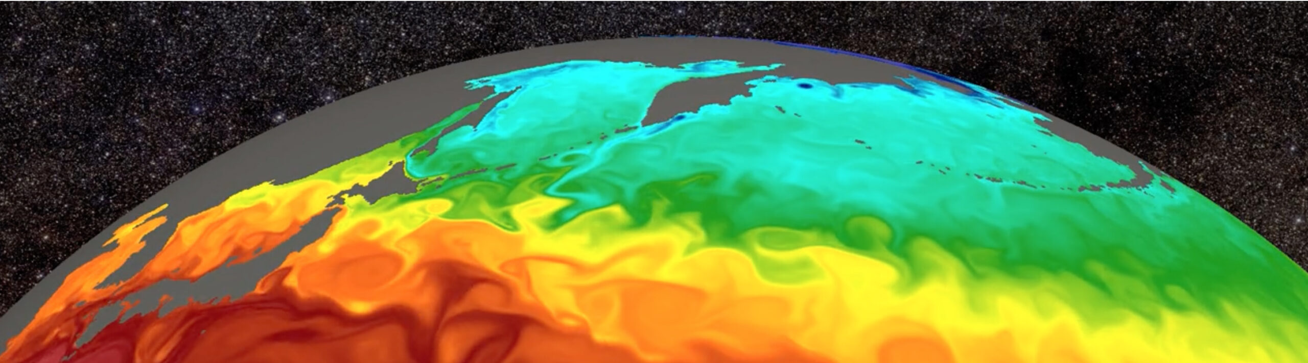
Earth Observation satellites generate massive volumes of data about our planet, and these data are vital for confronting global challenges. Satellite imagery is commonly distributed as individual “scenes” — a single file consisting of a single image of a tiny part of the Earth. Popular public satellite programs such such as NASA / USGS Landsat and Copernicus Sentinel produce millions of such images a year, comprising petabytes of data.

Increasingly, we see organizations looking to aggregate raw satellite imagery into more analysis-ready datacubes. In contrast to millions of individual images sampled unevenly in space and time, Earth-system datacubes contain multiple variables, aligned to a uniform spatio-temporal grid. Data cubes are great for applications that go beyond just looking at a pretty picture of the Earth, including statistical analysis, assessing changes and trends, and training predictive models. (A great overview of Data Cube technology and applications can be found in Mahecha et al., 2020.)

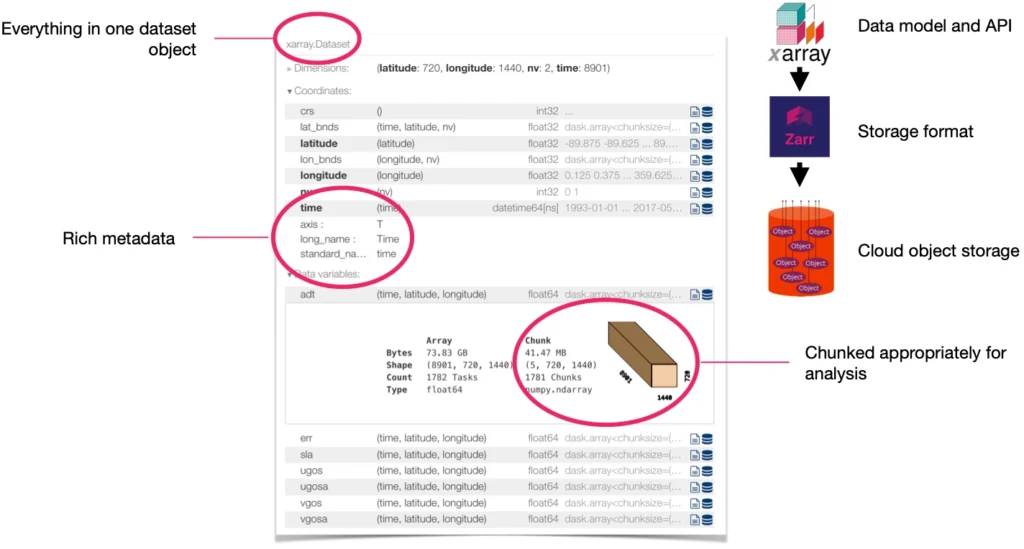
We’ve observed a growing number of organizations choosing to store their datacubes in the Zarr format—from public-sector organizations like ESA and NASA to innovative startups like Pachama and Sylvera (a valued Earthmover customer). As core developers of the open-source Zarr-Python library, and as the creators of Arraylake, the first cloud data lake platform based on the Zarr data model, we’ve been following this trend closely. Zarr is indeed a great choice for datacubes: it allows for storing multidimensional arrays (a.k.a. tensors) of unlimited size in a performant, cloud-optimized way. When paired with Xarray, you’ve got a powerful, flexible query engine for datacubes.

This blog post is our attempt to synthesize some of the best practices we’ve seen for how to build custom datacubes from EO data. We’ve had a lot of input from the community along the way (see Acknlowedgements section).

Building Blocks

Our task for this example is simple but representative of the basic datacube processing workflow. Starting from Sentinel-2 Level 2 imagery, stored as Cloud Optimized Geotiffs in the AWS Open Data program, we want to build a datacube over a large area with uniform spatial and temporal resolution. We will aggregate data in the time dimension over a customizable interval (here we’re using monthly), computing the median over each cloud-free pixel. To accomplish this, we will leverage the amazing capabilities of the open-source Python ecosystem, including pacakges such as Xarray, Dask, RioXarray, Rasterio, PySTAC, and Open Data Cube, and many more.

Intialize a Template Dataset

First we will define the target grid and structure for the datacube we want to produce. At this point we have to define several parameters, all of which are customizable:

• The spatial Coordinate Reference System (CRS) and resolution of our datacube. Here we are using a simple lat / lon grid (EPSG:4326) at 30 meter resolution, but this is customizable. (For a consideration of alternative choices, see discussion below.)
• The temporal resolution (here monthly). Ideally this should be long enough to find multiple cloud-free images per pixel. Shorter intervals give better temporal resolution of changes at the expense of increased noise and missing data.
• The bands we want to store. (Here just Red, Blue, and Green.)
• The chunking of the Zarr dataset. This is important, because it constrains how we will write our data. Here we are using chunks of 1200 x 1200 pixels as a default. Making these larger would require more memory in each task. Making them smaller would lead to a larger number of tasks.

To create this template dataset, we use the Open Data Cube odc.geo package. The code looks something like this

# create ODC geobox for the full cube extent
geobox = GeoBox.from_bbox(bounds, crs=crs, resolution=dx)
# create a big, empty Xarray dataset for this region
big_ds = (
    xr_zeros(self.geobox, chunks=-1, dtype="uint16")
    .expand_dims({"band": bands, "time": time_data})
    .transpose(..., "band")
).to_dataset(name="rgb_median")
# write the Zarr dataset schema and coordinates, but no data variables
big_ds.to_zarr(zarr_store, encoding=encoding, compute=False)

(The full code is a bit more complex, but this gets the point across.)

Here are a few of the advanced techniques we used in this step to optimize the creation of the schema and the storage settings of the variables:

• Optimize Zarr encoding for coordinates to achieve optimal compression.
• Using only one massive Dask chunk for the whole array to avoid unnecessary overhead. (We’re never going to compute it anyway.)
• Manually specify the Zarr chunks in encoding.

Compute a Single Chunk

Now we need to figure out how to supply the data for a single chunk. We can break this down into several steps. For each chunk, we must

• Find all of the individual scenes that intersect with the chunk’s bounding box. This is super easy thanks to the Element84 Earth Search service, which stores this information in a super-fast database that we can query via a STAC API.
• Align each scene to our target CRS and grid. odc.stac makes this a breeze.
• Aggregate the data temporally, using a mask to discard cloud pixels or other invalid data.
• Store this piece of data into our big Zarr array.

Throughout all of these steps, we use Xarray as the container for our data and leverage the Xarray API to express these steps in a clear, concise syntax. You can see the full code to do this in our demo repo. It’s about 100 lines of generously spaced, fully typed Python

⚠️ Now for a disclaimer: The “right way” to do cloud masking and temporal aggregation to produce a cloud-free mosaic is a complex scientific problem. People write whole PhDs on this topic. There are much more sophisticated algorithms and approaches than the one we are using here. The code we are sharing is a simple starting point, but most serious users will want to customize this step considerably.

We had to call this function lots of times, so it was worth spending some time to optimize it (with lots of help from the Pangeo community). Some of the tricks we used to speed things up are as follows:

• Use a rasterio configuration optimized for cloud. Specifically, odc.stac.configure_rio(cloud_defaults=True, aws={"aws_unsigned": True}).
• Tune our chunking in odc.stac.load. We settled on chunks={"time": 1, "x": 600, "y": 600 with low conviction.
• Oversubscribe the Dask threadpool in order to maximize I/O throughput. We landed on 16 threads, even when running on a virtual machine with only 2 cores.
• Write the data directly with the low-level Zarr API (rather than Xarray) in order to minimize unnecessary metadata and coordinate operations. (This came with the tradeoff of more verbose code and brittle indexing logic.)

In the end, for a 1200 x 1200 pixel chunk, aggregating over 20-30 scenes, we could run the whole thing in around 20s. (Our original implementation was more like 1-2 minutes.)

Enumerate All Chunks and Discard Ocean

To build our datacube, we need to repeat this step over and over for every chunk. However, since we’re focused on the land surface, we don’t care about loading data over the ocean and can save some time by discarding chunks that don’t intersect with land. (As a card-carrying oceanographer, this step breaks my heart a little. 🥲)

We need a function that, given a particular chunk, can quickly determine if that chunk is pure ocean. For this, we used Cartopy’s LAND feature, a convenient packaging of the Natural Earth Land vector dataset into Shapely geometries. The check is just a few simple lines of code.

bbox = tile.boundingbox
extent = bbox.left, bbox.right, bbox.bottom, bbox.top
igeoms = list(LAND.intersecting_geometries(extent))
is_land = len(igeoms) > 0

Honestly, the hardest part here was figuring out how each different package wanted to express the bounding box rectangle around a region! Can’t we just pick one convention and stick to it? 😆 Or, better yet, develop tools that natively understand such concepts at a high level and communicate automatically.

Anyway, with these building blocks in place, we’re ready to scale up!

A Serverless Approach

A naive approach to building the full datacube might look like this—a giant for loop:

for chunk in all_chunks:
    populate_data_for(chunk)

At that rate, it would take a couple of days to create a datacube at the country scale. However, we can quickly realize that this problem is embarssingly parallel; there are no dependencies between chunks. So rather than computing chunks one at a time, we can do them all at once. This sort of problem is a great fit for serverless computing.

Serverless computing is a cloud computing approach in which the user doesn’t have to think about or manage any backend servers, clusters, or other infrastructure. Instead, the user just defines a function they want to execute in the cloud and then calls this as many times as they want. It’s the cloud-provider’s job to figure out how to scale up the resources. As someone who has spent too many precious hours wrestling with servers and clusters, I can say definitively that I find serverless computing to be a joyful developer experience, particularly given the latest crop of serverless frameworks (more below).

Conceptually, what we want to do is illustrated by the diagram below:

This approach requires a “coordination node” which is responsible for initializing the target Zarr dataset, spawning each individual chunk processing job, and then waiting for them all to finish. Here I just used my laptop as the coordination node; however, for a more automated approach, you could integrate this into a CI/CD pipeline (e.g. GitHub workflows) or an orchestration framework (Airflow, Dagster, Prefect, etc.).

Our Application Structure

We developed our demo application as a click CLI tool. Here’s the basic file structure:

└── src
    ├── main.py
    ├── lib.py
    ├── storage.py
    ├── coiled_app.py
    ├── modal_app.py
    └── lithops_app.py

We call it from the command line and pass all of the parameters (spatial bounding box, temporal extent, resolution, bands, target location, etc.) as arguments. The command parsing logic lives in main.py. All of the “business logic” of our application (initializing the datacube, querying the STAC catalog, writing the data, etc.) lives in lib.py.

To enable us to try this approach with different serverless frameworks, we implemented a common interface to three different frameworks. From main.py, we just have to call

spawn(jobs, target_array)

and the jobs get launched against our desired service. We also abstracted the storage layer to work both with vanilla object storage and with Arraylake, our data lake platform which specializes in storing Zarr data. These abstractions allowed us to easily compare these different technology choices.

An example invocation of this command-line application, which builds a baby datacube over my home state of Vermont, looks like this:

python src/main.py \
--start-date 2020-01-01 --end-date 2023-12-31 \
--bbox -73.43 42.72 -71.47 45.02 \
--storage-backend arraylake \
--arraylake-repo-name "earthmover-demos/sentinel-datacube-Vermont" \
--serverless-backend lithops

Serverless Frameworks

Serverless has gotten a lot easier than it used to be. The industry-standard serverless framework is AWS Lambda. While highly scalable and reasonably cost effective, Lambda is notoriously hard to configure and develop against, particularly in the sort of iterative, interactive way that most data scientists and engineers like to work.

We developed our demo application to run against three different serverless frameworks:

1. Coiled Functions - a new offering from Coiled, the company behind Dask.
2. Modal - a new serverless platform for AI and Data teams.
3. LithOps - a new open-source project which provides a uniform API for serverless applications to run against cloud-provider offerings like AWS Lambda, Google Cloud Functions, etc.

All of these platforms offer the ability to define functions locally and run them remotely in an easy, developer-friendly way. I wrote my code in VS-Code on my laptop, and it ran in the cloud. Magic! 🪄

On a basic level, all three of these frameworks got the job done. 💪

Beyond that, there were some noteable differences and tradeoffs between them. Here’s a quick summary of the pros and cons we found with the different frameworks.

Lithops + AWS Lambda Executor

Modal

Coiled Functions

The speed of serializing spawning tasks turned out to be the main bottleneck limiting our ability to scale. This was directly tied to how each framework serailized our local code and shipped it up to the serverless runtime. Both Lithops and Coiled Functions had a relatively high overhead associated with this step. Modal, instead, has some special sauce that does this just once for our app, allowing it to spawn tasks at a much faster rate. For this reason, we preferred Modal for our largest (continental scale) datacubes with hundreds of thousands of tasks. We could likely overcome this difference by packaging all of our code into a pip or conda package, rather than relying on local modules; however, that would really slow down the developer experience, requiring us to push code to github or pypi every time we wanted to tweak the logic.

The Arraylake Advantage

We also had a chance to compare storing our Zarr datacube in Arraylake vs. just dumping it into raw cloud storage. We were inspired to build Arraylake based on our past experience of managing large-scale Zarr datasets in the cloud. It’s a purpose-build platform that solves all of the common challenges that teams encounter when working with Zarr data pipelines at scale.

Not surprisingly, it was much nicer using Arraylake compared to raw object storage! For starters, Arraylake automatically provides a clean web-based data catalog on top of our data. The ability to quickly see what data you have in the web, rather than having to use Python or a CLI tool, really improves the developer experience.

However, the killer feature of Arraylake in for this application is its support for ACID Transactions. In the course of building this pipeline, we experienced frequenct failures and errors. This is par for the course when prototyping a new data pipeline! When pipelines fail, the Zarr data can be left in an ambiguous, possibly inconsistent, possibly corrupted state. When working directly with object storage, that state is permanent. However, because Arraylake support atomic commits across long-lived distributed sessions, you can easily roll-back any changes if the pipeline fails. By only committing once the pipeline has succeeded, you are guaranteed that only correct, clean data is available to you users. This is crucial for any team using Zarr in production!

A Sample Run

To visualize how the work happens in this serverless pipeline, we can take advantage of Lithops excellent built-in visualization of execution stats. Here’s a timeline view of the execution of a run with 1000 tasks:

All 100 tasks all start within 5 seconds of each other. Most finish within 20-30 seconds, although there are a few outliers that take up to a minute. We configured our tasks with a timeout of 90s; after this, they will give up and retry 5 times before failing. There are lots of sources of variability and potential failure along the way, including the STAC API call, the reads from S3, and the writes to the target store. We experienced random errors or timeouts about 1 in 10,000 tasks we ran, and a single retry was usually enough to move forward.

Costs

It’s shocking how cheap this is. Here is a screenshot of the AWS cost analyzer for Lambda for one run of a pipeline with 6643 chunks.

Coiled Functions was in the same ballpark. Modal was about 100x more, coming in at around $100.

Because of this, we spent zero time trying to optimize for costs. It’s likely that each serverless runtime could be optimized considerably to reduce costs further.

One non-obvious conclusion from this is that the main cost in this type of workflow is developer time. I probably spent about 10 hours developing this demo. At a typical developer rate of $100 / hour, that’s $1000, orders of magnitude more than the compute costs themselves. It’s striking how often teams seem to overlook this aspect when considering the value of products and services. Investments in developer tools that increase productivity are probably the greatest opportunity for cost savings in this domain.

The Final Product

After everything is deployed and tuned, we have the ability to run a simple command-line script and produce a massive-scale datacube in the cloud, all from our laptop. Honestly, this feels like a super power.

Here’s an example of one of the mosaics we built over South America. Stored in Arraylake, opening the datacube is trivial.

client = arraylake.Client()
repo = client.get_repo("earthmover-demos/sentinel-datacube-South-America")
ds = repo.to_xarray(mask_and_scale=False, chunks={})

We can easily pull out and plot locations of interest, for example, this beautiful view of the Atacama desert.

# mask invalid pixels with NaNs
rgb = ds.rgb_median
valid = rgb>0
rgb = rgb.where(valid)

# pull out the data we want
patch = rgb.sel(latitude=slice(-24, -25), longitude=slice(-70, -69)).load()

# plot with matplotlib
fig = plt.figure(figsize=(14, 10))
ax = plt.axes(projection=ccrs.PlateCarree())
patch.squeeze().plot.imshow(rgb="band", ax=ax, robust=True, transform=ccrs.PlateCarree())
ax.gridlines(draw_labels=True)

We can also use this dataset as the data source for an AI/ML training pipeline, as explained in our recent blog post Cloud-native Data Loaders for Machine Learning using Zarr and Xarray.

What Could be Improved?

We’re pretty happy with how this worked. We now have the ability to very easily build custom datacubes for regions of interest, storing them as analysis-ready Zarr datasets directly in object storage or in Arraylake. The serverless runtimes all scale out extremely well and are very cost effective. Yay! 🎉

The Zarr datacubes are excellent for analytical and machine-learning workflows that need to efficiently access and process the data. However, we also noticed several areas where storing datacubes in Zarr still feels sub-optimal. These are areas where our community can focus future development effort.

• Visualization - It’s hard to visualize the data stored in Zarr in a traditional “slippy map”. The best we can do is load the data into Python and plot it with Matplotlib / Cartopy. This can come as a shock to many GIS-type users, who have come to expect that sort of interactive data visualization experience.

  There are two paths forward that could help improve this situation.

  • Direct visualization of Zarr in the browser, i.e. pointing a browser-based tool directly at Zarr data in object storage. This is already somewhat possible today, thanks to CarbonPlan Maps. However, CarbonPlan Maps only work with a very specific data profile, which includes a multiscale image pyramid and a Web Mercator CRS. Our datacubes don’t conform to this requirement. Going forward, we’re optimistic that the GeoZarr Specification (currently under development) can have a big impact here by standardizing how geospatial raster data is stored in Zarr. This should allow visualization tools to work better with Zarr-based datacubes.
  • Server-proxied visualization. This means having some sort of compute in between the browser and the raw Zarr data. For example, a dynamic tile server like TiTiler could read the Zarr data and generate map tiles on the fly. These maps tiles could then be used in any standard GIS map environment. Another interesting possibility in this space is Fused, a new serverless platform for geospatial transformation and visualization.

• Choice of Grid and CRS - Our choice of EPSG:4326 (i.e. simple lat / lon grid) is convenient when paired with Xarray. Xarray’s dimension-based indexes allow us to easily query and subset based on lat, lon, and time. However, if you consider this as a map projection, it has some drawbacks on a global scale. Specifically, this is not an equal-area grid—the grid points near the poles are significantly smaller in area than the ones near the equator. For applications focused on low-latitudes (e.g. tropical forests), it’s probably fine. Some alternatives we could consider are:

  • Using a regional CRS for a regional-scale cube. For example, we could use the State Plane Coordinate System for US states.
  • Using a Discrete Global Grid System, such as H3 or Healpix. While DGGSs have traditionally be used more for vector data aggregations, they should also work great with datacubes. The Pangeo Community has been discussing how to integreate DGGSs with Xarray. The result of this is the newly created xdggs package. We’re looking forward to helping this package grow and mature!

We learned a lot from this experiment, and we hope you learned something from the blog post. We’re excited to work with the rest of the Earth Observation community to improve how we create and manage analysis ready datacubes. Let us know what you think of this approach in a comment on LinkedIn or Twitter.

Acknlowedgements

• Copernicus Program for the Sentinel Satellites
• AWS for the Open Data Program
• Cloud Native Geospatial Community for COG and STAC
• Element84 and Development Seed for running expensive public STAC API endpoints
• Pangeo Community for Xarray and Zarr
• OpenDataCube Community for great ODC tools
• Alex Leith & Kirill Kouzoubov in particular for their help
• Sylvera for the inspiration to explore this topic
• Lithops, Modal, Coiled for making serverless easy

References

1. Mahecha, M. D., Gans, F., Brandt, G., Christiansen, R., Cornell, S. E., Fomferra, N., Kraemer, G., Peters, J., Bodesheim, P., Camps-Valls, G., Donges, J. F., Dorigo, W., Estupinan-Suarez, L. M., Gutierrez-Velez, V. H., Gutwin, M., Jung, M., Londoño, M. C., Miralles, D. G., Papastefanou, P., and Reichstein, M.: Earth system datacubes unravel global multivariate dynamics, Earth Syst. Dynam., 11, 201–234, <https://doi.org/10.5194/esd-11-201-2020>, 2020.