At Earthmover, we are building the cloud platform for multidimensional array data (a.k.a. tensors). While the need for such a platform is obvious to practitioners in weather, climate, and geospatial data science (not to mention AI, where tensors reign supreme), folks from the mainstream data world often ask, why don’t you just convert everything to tabular? Indeed, in certain corners of the internet, one gets the impression that cloud data management and analytics is basically fully solved by technologies like Parquet, Arrow, DuckDB, etc. (For example, nothing about array or tensor storage appears at all on Bessemer’s Roadmap: Data 3.0 in the Lakehouse Era.)

This post explains why we need Array-native data systems from first principles. It’s aimed at a technical audience familiar with mainstream tabular data systems but new to the world of array-based data systems.

Defining “Structured Data”

At the crux of this issue is what it means for data to be “structured.” Today, structured data is typically understood to be tabular, organized into rows and columns, and compatible with the relational data model used ubiquitously in database systems.

But let’s go a bit beyond this conventional definition and think about what “structured data” really means. At its essence, structured data is data that conforms to some sort of pre-defined data model, which we can leverage to improve both the efficiency of storage and the performance of queries. The relational model is one such example of a data model.

As a simple example, consider the following data about planetary masses stored as JSON (technically a “semi-structured” form)

[
	{
		"name": "Mercury",
		"mass": 3.00e23
	},
	{
		"name": "Venus",
		"mass": 4.87e24
	},
	{
		"name": "Earth",
		"mass": 5.97e24
	},
]

vs. CSV (a structured form)

name,mass
"Mercury",3.00e23
"Venus",4.87e24
"Earth",5.97e24

It’s obvious that the CSV representation is both more compact (fewer characters) and more efficient to scan / process. That’s because the JSON version has redundant information (column names repeated in every item) rather than just in the header like CSV. This is the key point, and a useful working definition: structured data employs a data model which eliminates all possible redundant information.

Of course, compression can also be used to eliminate redundant information. However, the data model is more fundamental. We could apply the same compression algorithm (e.g. ZSTD) to both the CSV or JSON data. A good compression algorithm will discover redundant information in the data and eliminate it; however, when it comes time to actually process the data, we have to reverse this process by decompressing. In contrast, the “compression” we get by using a structured data model is much more useful for analytics than just blindly applying a compression algorithm. State-of-the-art formats like Parquet and Zarr use both approaches; structured data are stored in a compact binary columnar layout, with encoding and compression applied to each column / variable chunk separately.

Below we will explain how multidimensional arrays are less redundant at the data-model level–and therefore more performant for common workloads involving gridded data.

Multidimensional Arrays and the NetCDF Data Model

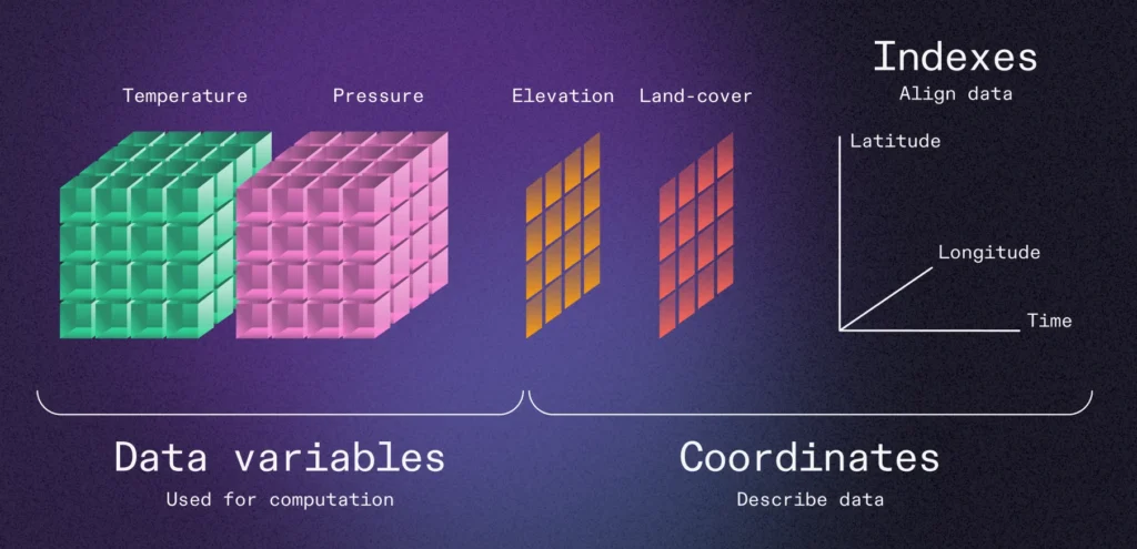
In the scientific data space, we have a well-established data model: the Unidata Common Data Model (CDM) (which builds on the NetCDF file format). While this data model is most prevalent in the geosciences, it can be applied to a wide range of science and engineering domains. The data model consists of one or more variables, each of which is a multidimensional array (tensor) with a homogeneous data type (e.g. float32) and named dimensions (e.g. x, y, time). Coordinates variables can [optionally] be used as indexes to [geo]locate data within other data variables. Xarray has a nice illustration of this data model:

There are exabytes of NetCDF / CDM data out there in the wild.

A NetCDF dataset is conceptually similar to a table, with the variable analogous to the column. However, there are two key differences.

• NetCDF variables are multidimensional arrays, while table columns are essentially one-dimensional arrays.
• Not every array is the same shape. Arrays can share dimensions, but not all dimensions need to be present in every array. (This is often the case with coordinate variables)

The latter property is a key optimization which eliminates a huge amount of potential redundancy. Consider a typical 2D array of temperature on a regular lat / lon grid. The NetCDF data model allows us to represent this in the following way, using one data variable and two (smaller) coordinate variables.

(The assumption here of course is that the dimensions are orthogonal to each other. Fortunately, that’s very often the case for data about the physical world. We live in a four-dimensional universe.)

In this model, the coordinates for the dimensions are stored in a very parsimonious way. Specifically, the number of cordinate values we store is just the sum of the length of each dimension. (Let’s call this number Nc.) It’s hard for Nc ever to become a big number. To use a common example from weather forecasting, Earthmover’s sample NOAA GFS dataset has dimensions of (longitude: 1440, latitude: 721, time: 1111, step: 209), consisting of over 5TB of data. But there are only 3481 total coordinate values (less than one MB of data).

One of Xarray’s many clever innovations was to turn these coordinate variables into in-memory indexes to facilitate selection of data. Because the coordinate variables are usually so small, it’s reasonable to read them into memory eagerly upon opening a dataset. Such indexes are also extremely efficient. The computational complexity of locating a particular point within an array using orthogonal indexes is just O(Nc). That’s because we can scan each index separately to locate a point within the full N-dimensional space. And unlike hierarchical multi-indexes, there is no inherent ordering to the dimensions to worry about.

So for multidimensional array data with orthogonal coordinates, we can see that the NetCDF data model has no redundant information stored and also supports a very efficient form of indexing within the coordinate space. Now what happens when we abandon the array data model and try to squeeze this type of data into a table?

The High Price of Flattening

Flattening multidimensional data can be thought of as “unrolling” each array into a single column, producing a standard tabular structure of columns and rows. For a data variable like temperature, this doesn’t change the number of elements; just the shape. Elements that were near each other in multidimensional space can end up very far apart in flattened space.

This flattening has a much more drastic effect on the coordinate variables. The coordinates must be duplicated over and over with repeated values in order to produce all of the correct coordinate / data tuples, as illustrated below.

Now the number of coordinate values we have to store increases as the product of the dimension sizes. This math causes the amount of coordinate data stored to explode, particularly as the number of dimensions increases. For the 4D weather forecast dataset described above, this means storing 964,313,159,040 coordinate values (compared to just 3481 in the NetCDF model). And we could easily introduce additional dimensions to the dataset (e.g. vertical level, ensemble member) which would further multiply this number!

Since many of those values are repeated, this redundant storage of coordinates can be mitigated with compression. However, it can’t be removed at the level of the data model. With the tabular structure, in order to locate a particular point in space / time, we must scan every single row. This has direct and unavoidable consequences for the performance of queries, as we will see below.

Benchmark: Xarray + Zarr + Icechunk vs. DuckDB + Parquet

To illustrate these consequences, we conducted a straightforward benchmark comparing the array-native data stack (Xarray + Zarr) to a state-of-the-art tabular stack (DuckDB + Parquet) for typical queries related to weather forecast data.

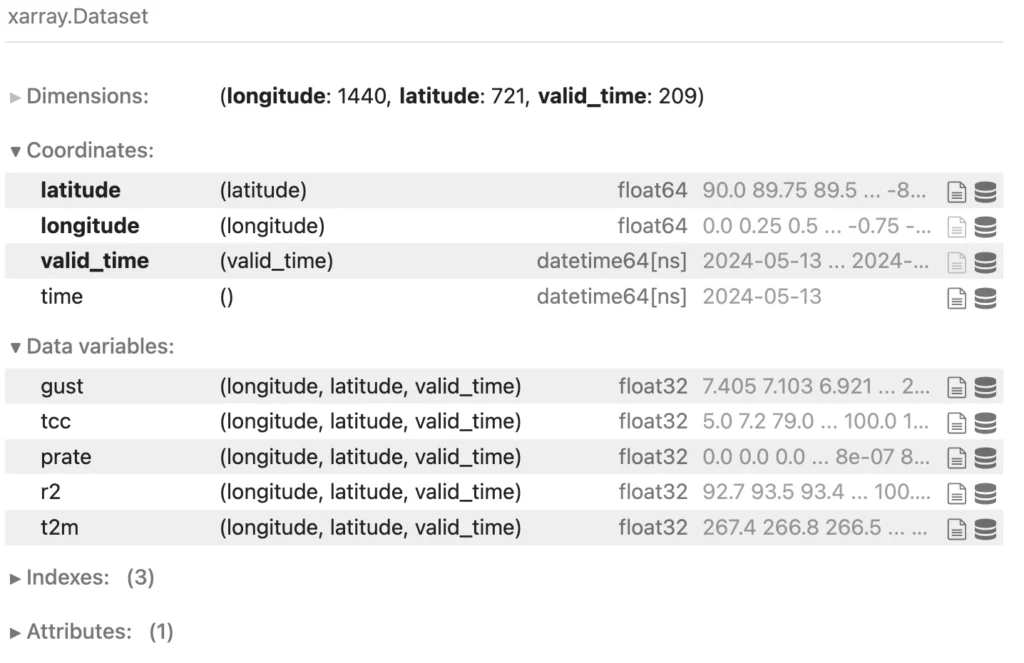
For our test dataset, we took a single forecast from the GFS dataset described above. Each forecast has hourly temporal resolution going out two weeks. We only consider surface data for this experiment. For our test dataset, we selected temperature, humidity, precipitation rate, total cloud cover, and gustiness–all variables relevant for renewable energy forecasting. The resulting Xarray dataset looks like this: five three-dimensional data variables, plus three one-dimensional coordinate variables (latitude, longitude, and valid_time). That’s about 4GB of uncompressed data.

We wrote this dataset to Zarr using Earthmover’s new Icechunk storage engine. Data variables were chunked with a fairly isotropic chunking scheme (360, 120, 24) and compressed using PCodec. To produce a tabular version of the dataset, we converted the Xarray dataset to a Pandas dataframe. We also transformed the latitude and longitude columns into a proper geospatial geometry column using GeoPandas. We then used GeoPandas to write a GeoParquet file with 8 columns and 216,992,160 rows using default encoding and compression. All data were stored in S3 and queried from an in-region EC2 instance–Xarray to query the Zarr and DuckDB to query the Parquet. (Check out the simple Jupyter Notebook used to produce the results shown below.)

It’s worth noting just how similar Xarray and DuckDB look in this context; they are both playing the role of an embedded analytical database engine. There is no database server; just a client process (in EC2) and the data files (in S3). The user expresses a query (in SQL for DuckDB; in Xarray’s dataframe-like API for Xarray), and the engine does its best to get the result as fast as possible. DuckDB is written in C++ and contains all of the latest academic innovations and optimizations for analytical query processing. It is frequently at the top of benchmarks for analytical query performance, so we expect it to be as fast as possible, given the constraints of the data model and data format.

There are multiple ways to slice this forecast. A common example is to extract a timeseries of temperature (the t2m variable) at a single location. This is what such a query looks like in Xarray:

ds["t2m"].sel(longitude=-105, latitude=40)

Here’s what the same query looks like in SQL against the GeoParquet data.

SELECT valid_time, t2m FROM forecast_data WHERE geometry=ST_Point(-105, 40)

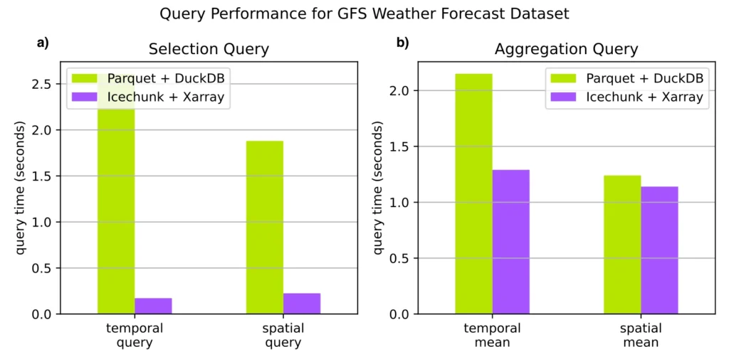
Xarray is able to compute the timeseries query in less than 200 ms. In contrast DuckDB takes over 2.5 seconds, more than 10x slower.

Another common query is a spatial query–extracting a single snapshot of the global forecast. In Xarray this is:

ds["t2m"].sel(time="2024-05-13:03:00:00")

In SQL this looks like:

SELECT geometry, t2m FROM forecast_data WHERE valid_time=make_timestamp(2024, 5, 13, 0, 3, 0)

This takes Xarray 225 ms, but nowhere close to DuckDB’s 1.9s.

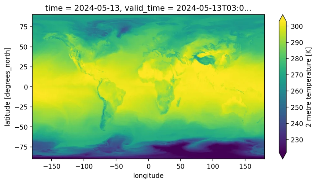
In addition to the major qualitative difference in performance, there’s an important quantitative difference highlighted by the spatial query. The result of the Xarray query is itself a coordinate-aware array, in this case a 2D lat-lon map, which we can trivially visualize, or continue to slice / process in an array-native way.

In contrast, the result of the spatial query in DuckDB is a dataframe of 1,038,240 individual points. I have no idea how to put them back together (i.e. “unflatten” them) to make a rectangular image. (If you do, please let me know in the comments!) While I suppose I could visualize them as vector data using a tool like Lonboard, this would be less efficient because we have discarded the inherent structure in the data.

It’s fair to say that this selection query, which involves minimal actual computation, does not play to DuckDB’s strength as an analytical processing engine. (It was designed to highlight the consequences of the different data models.) So let’s try something that requires more computation. Now, instead of selecting a single timeseries, we’ll a) compute the mean over every single point in space (a spatial mean) and b) compute the temporal mean at each point. These are two common aggregation-style processing tasks for weather data. This is what these queries look like in Xarray.

spatial_mean = ds["t2m"].mean(dim=("longitude", "latitude"))
temporal_mean = ds["t2m"].mean("time")

In SQL, we have to implement these aggregations as a groupby operation.

-- spatial mean
SELECT AVG(t2m), valid_time FROM forecast_data GROUP BY valid_time;
-- temporal mean
SELECT AVG(t2m), geometry FROM forecast_data GROUP BY geometry;

In this case the entire variable / column has to be read. For the spatial mean, Xarray and DuckDB are on par, while for the temporal mean, Xarray is nearly 2x faster. Our hypothesis for why is that the on-disk and in-memory layout of the data–as arrays–is optimized to support reduction over the dimension axes. Instead, DuckDB must do an expensive groupby in order to reconstruct the original structure of the data.

These simple benchmarks clearly illustrate what we expected from the first-principles approach. Organizing array data with orthogonal coordinates into the NetCDF data model leads to efficient storage and queries. Flattening such data into a tabular form induces a significant performance and usability penalty. We see no advantages here to using a tabular stack.

This was a modest-sized example (three-dimensions, 4GB of data). Increasing the size and dimensionality of the data only exacerbates the performance penalty.

“Tensors as Columns” vs. “Tensors inside Tables”

There is a partial analogy between NetCDF (tensor) variables and columns–they each represent distinct attributes of the same dataset. But the array-based NetCDF data model is fundamentally incompatible with the tabular data model–in the Arrow data model, for example, each column is stored as a one-dimensional Arrow Array, while NetCDF variables are N-dimensional.

However, Arrow and other tabular technologies do have some integration with tensors which muddy the waters a bit around this issue. Arrow and other databases do permit you to put tensors inside tables. An individual value can be a nested list, which can be decoded to a tensor, or a tensor using the fixed-shape tensor Arrow extension type. This allows you to store individual tensors within the rows / columns of a tabular data structure. However, the size of this tensor is obviously constrained; you would not want to store a massive, multi-TB array as a single tensor-encoded Arrow value. Instead, you would want to split up the tensor into smaller chunks…but how? Along which axis? And how do you keep track of the relationship between chunks? These are all questions that are answered by Zarr.

Similarly, many geospatial databases allow you to store raster data in a table (e.g. PostGIS, Apache Sedona). And there are efforts like Raquet which define a way to put raster data inside a Parquet file. In GIS world, a “raster” is understood to mean a single 2D rectangular image, potentially with multiple bands, and a spatial bounding box. These databases store the raster data, along with its bounding box and other relevant metadata, as a single row. There is no notion of a contiguous global domain. While this organization may be suitable for a Level 2 collection of satellite images, it’s redundant (and therefore, inefficient) for Level 3 data and beyond. Furthermore, adding additional dimensions (e.g. time, space) in this model is awkward.

To summarize: putting individual tensors inside tables is not the same as modeling your entire dataset as a collection of [potentially very large] contiguous tensors.

When to use Tensors vs. Tables?

For data that maps well to the relational data model, it makes sense to use tables. This includes most business data (orders, users, accounts, etc.)

For data about the physical world, including scientific data from sensors, imaging systems, satellites, the data originate in a three-dimensional universe (plus time) and therefore naturally conform to the more general NetCDF data model, in which orthogonal physical dimensions are preserved at the data storage level. Beyond weather data, geospatial raster data and data cubes are one obvious example. But this is also the case for any sort of physical simulation data, regardless of the spatial grid type (rectilinear grid, unstructured mesh, etc). For example, Azavea previously compared Zarr and Parquet for NOAA National Water Model data, which uses an unstructured mesh for the spatial coordinates. The resulting dataset had only two dimensions (time and feature_id), but Zarr was still 2-10x faster for their benchmarks.

The tensor model is also ideal for bioimaging data. The OME-Zarr standard defines profiles suitable for storing a wide range of microscopy datasets, including fluorescence imaging and whole-slide imaging. Zarr is also used extensively in neural imaging and neural connectomics.

Moving farther afield, we are seeing growing numbers of applications of this data model in drug discovery, molecular dynamics, autonomous vehicles, fusion and plasma physics, materials science, energy, and quantitative finance.

Do you have a novel use case for Zarr? Let us know in the comments!

What’s next for the Array Data Ecosystem?

While there’s clearly a need for tensor-specific data systems which understand the NetCDF data model, this area of technology undoubtedly remains much less mature than its tabular counterpart. This represents an amazing opportunity! Today, Xarray and its ecosystem (Zarr, Dask, etc.) is the most advanced and full-featured Array-based query engine. But there’s still so much to build! At Earthmover, we’re committed to investing in this stack and driving it forward with new innovation.

Fortunately, there are many great ideas from the tabular world that are ripe for transposition to the array world. As an example, our new Icechunk storage engine takes inspiration from Apache Iceberg and other modern table formats, introducing ACID transactions and data version control on top of the Zarr storage model. This innovation paves the way to true database-style interaction with Array data, where multiple readers and writers can all safely access the same dataset in cloud object storage. We’re excited to be working with a vibrant open-source array community to advance Icechunk and other transformative new technologies.

In stark contrast to tabular data, there are almost no commercial cloud infrastructure services aimed at array data, which places a huge burden on engineering teams in this space to build everything from scratch. The Earthmover Platform is an end-to-end cloud data management solution with a native understanding of arrays and the NetCDF data model. Our platform (built on the open-source core of Xarray, Zarr, and Icechunk) supports teams across the full lifecycle of scientific data, from research and prototyping to delivery of production data via standards-compliant APIs without having to set up and maintain complex infrastructure.

We’re passionate about helping real scientists and developers faced with hard data problems in the physical world: from weather forecasting, to monitoring deforestation, to modeling fusion. To support these critical applications and many more, we need to ditch tables and put arrays front and center in our data systems!